


Special Article
Chapter 1,
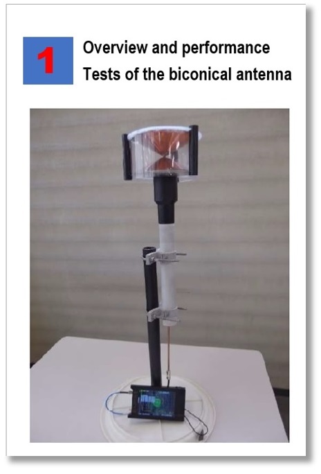
Overview and performance tests of the biconical antenna
What is a biconical antenna?
Due to the very short wavelength of the SHF bands, and the nature of the radio waves used, you will often see pictures of SHF band transceivers being operated with parabolic antennas with gain. Since I am a beginner, and not familiar with the SHF band, I decided to focus on an omni-directional biconical antenna since building a parabolic antenna is a hurdle and I have no one to communicate with on a pinpoint basis.
Biconical is a combination of the words bi, meaning "two," and conical, meaning "having the shape of a cone.” The shape of the antenna is shown in Figure 1, with the vertices of each cone facing each other.
The basic shape is a dipole antenna. In a biconical antenna, the element part of the dipole is not a line like a wire, but has an area or volume as shown in Figure 1. This is effective in frequency bands with wide bandwidths, such as the SHF bands.
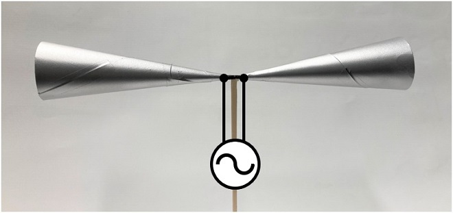
Figure 1. Model of a horizontally polarized biconical antenna made from cardboard.
The antenna is also said to be generally resistant to fading and other characteristics. It may be effective not for communications between fixed stations, but for communications with moving stations.
Concerning coaxial cable loss in antenna building.
One of my concerns during building was the loss in the coaxial cable. Coaxial cable is used to connect the antenna to the transverter directly below it, but since the frequency used is 5.7 GHz, even a short coaxial cable of about 50 cm may cause significant loss. Table 1 shows data obtained from a friend that examines the loss of Teflon coaxial cables and semi-rigid cables, although the data is specific to the amateur bands in the SHF band. The loss of both cables increases as the frequency increases.
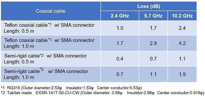
Table 1. Losses in the SHF bands for Teflon coaxial and semi-rigid cables
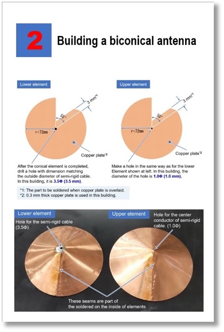
There are other coaxial cables with very low loss and high performance used in RF measurements, but I cannot afford them. The data in Table 1 show that at such high frequencies, even a 50 cm coaxial cable has more loss than expected and cannot be ignored. Therefore, I decided to use a semi-rigid cable with an outer conductor made of a metal tube to reduce the loss as much as possible. As described later in the antenna building section, the antenna element and the semi-rigid cable are made as a single piece.
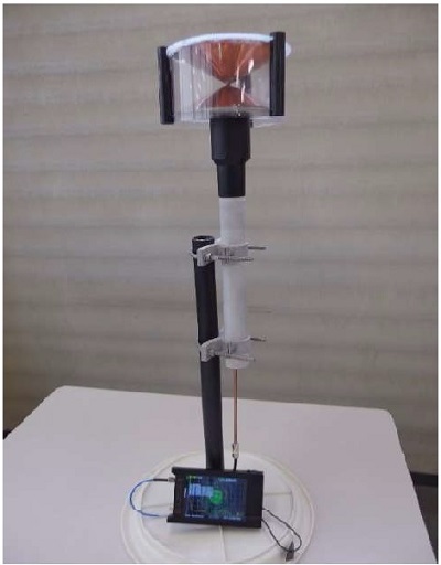
Appearance of the Biconical antenna.
Figure 2 shows the completed vertically polarized biconical antenna. It differs slightly from the model cone shown in Figure 1, but the basic conical elements are the same. Since the antenna is a prototype, I have not considered any degradation of the resin due to ultraviolet rays when exposed to sunlight for a long period of time, but I have added a simple structure to ensure waterproofing and wind resistance.
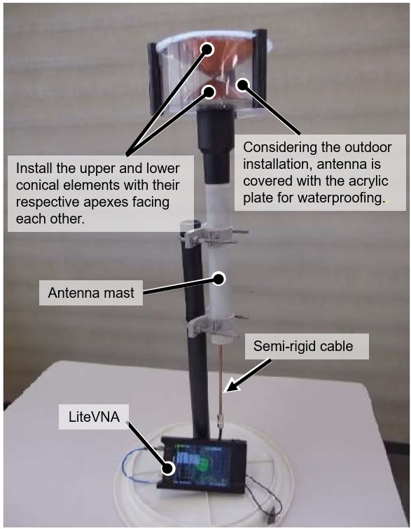
Figure 2. Completed biconical antenna (vertically polarized)
Performance of the built biconical antenna.
The LiteVNA was connected to the biconical antenna shown in Figure 2 through a semi-rigid cable feed line. I had no choice but to fully rely on the displayed values, as the LiteVNA is the only instrument I have that can measure up to 5.7 GHz. The project was a trial and error process, and Figures 3 and 4 show the results.
(1) SWR Characteristics
You can see that the SWR is 1.459 when the frequency is 5.77 GHz on the display shown in Figure 3. Although I would like to fully trust the displayed value, I am also concerned about accuracy of that values. So, I asked a third party to perform the measurement using a high-precision network analyzer for RF circuit design.
The result is the graph shown in Figure 4. The graph on the right side of Figure 4 shows the SWR characteristics: at 5.7 GHz, the SWR is displayed as 1.40, which is almost the same value as the 1.459 value measured by LiteVNA at 5.77 GHz. This seems to indicate that the data displayed by LiteVNA is reliable.

Figure 3. Observing the performance of a biconical antenna with LiteVNA
(2) Return Loss
The graph on the left side of Figure 4 shows return loss. It is the ratio of reflected power to forward power. Although the frequencies vary widely, it can be seen that the reflected power is almost constant at -15 dB to -16 dB relative to the forward power from the 2.4 GHz band to the 10 GHz band.
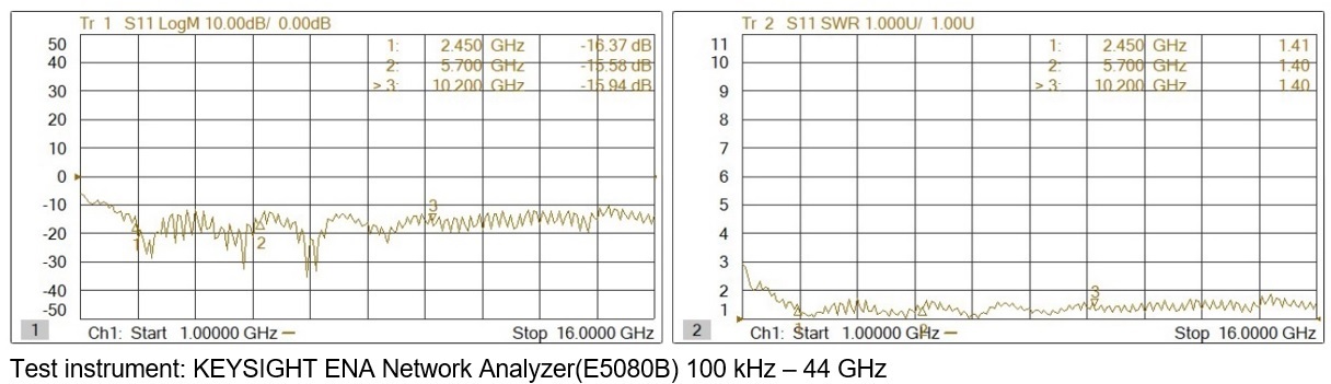
Figure 4. Performance tests using a high-precision network analyzer
(3) Vertical Plane Pointing Characteristic
Discone antennas are well known as broadband antennas, and the wider the angle of the cone (conical part), the wider the bandwidth. But on the other hand, the launch angle of the vertical directivity is slightly lower than the horizontal. The vertical plane directivity is almost horizontal because the top and bottom elements are the same cone in the case of a biconical antenna.
I measured this in a simple way in a shielded room. Figure 5 shows the directivity characteristics. Although the measurement data is very rough, it shows that the radio waves radiated from the biconical antenna are oriented horizontally to the ground.

(4) Summary of Electrical Performance
Table 2 summarizes what the graphs in Figure 4 and Figure 5 show. The graph in Figure 4 shows that while the frequency has changed significantly from 2.4 GHz to 10 GHz, there has been almost no change in return loss and SWR characteristics. The same is true for the vertical plane directivity characteristics shown in Figure 5.
It appears that the prototype antenna can be used not only for the 5.7 GHz band, based on this data, which was the target of this project, but also for the bands above and below that band.
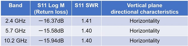
Table 2. Summary of measured data
Jump to the page you want to read when you click a picture above.