In Part 1 of this article, I noted that external antenna tuning units (ATUs) are a very popular station accessory, but they do not actually tune the antenna. They only transform the impedance at the end of the feedline to the transmitter’s output impedance so it can deliver maximum power, so they really should be called matching units. I showed that remote matching (at the antenna) has an advantage over matching in the shack because it reduces VSWR over the entire length of the feedline.

In this final part I explain why I built a remote matching unit, how I used simple software to design it, and the many mistakes I made before I got a working product.

Some background

I have a sentimental attachment to the 7 MHz (40-meter) amateur band. My first QSO as Novice KN2RDP in 1957 was on crystal frequency 7156 KHz. I became inactive in 1969, but 45 years later I was back on the air in Okinawa using a FT-101ZD that had belonged to JA9BB, my wife’s (SK) father. As the sunspots disappeared, I found 7 MHz was still good for both DX and local contacts. I built several antennas, finally keeping a 1/4-wavelength vertical ground plane (VGP) with elevated radials, and a full-wavelength vertical delta loop. They are about 15 meters above ground level and get strong DX signal reports. I can use them as a phased array for directional gain, and over the years more HF and VHF/UHF antennas joined them on the roof.

Most amateurs like to operate on several HF bands to take advantage of varying conditions. I wanted to use 3.5 and 10 MHz but had no space for more antennas. There are several ways an antenna originally built for one band can be used on others. These methods have been used for many years by amateurs and in commercial multi-band antennas, but often require an ATU to overcome impedance mismatches. Getting some wire up in the air is the most important thing, and we joke that our ATUs can match bedsprings, lawn chairs, or the proverbial wet noodle. Most hams are happy to get low VSWRs at the rig, and go on making contacts without thinking about feedline losses.

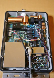
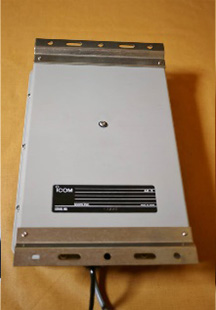
Fewer hams use remote ATUs (Figures 1a and 1b), which actually can reduce feedline loss. These are usually the automatic type and must be weatherproof, so cost more than desktop units, especially if rated for high power. I thought I could make a simple high-power matching unit out of parts I already had and protected by an outdoor electrical box.

The design begins with software

Transmission lines and matching networks for RF are described by relatively simple mathematical formulas. Before computers, they were usually designed by engineers, but now the formulas are embedded in online calculators that require little knowledge to use. Matching units at the base of a vertical antenna can provide multi-band operation, with some using separate networks switched by relays. I liked that approach, but I had to decide which antenna would be more suitable. Modeling programs that make thousands of iterative calculations are used to design and compare antennas. They were impractical before computers, but now we can have sophisticated software like EZNEC, 4NEC2, and MMANA-GAL on our PCs. I used the latter to compare my two 7 MHz antennas for use on the other bands. Its library already included both antenna designs.

Figures 2a and 2b. MMANA-GAL calculations for the vertical delta loop

The model showed that the 7 MHz Delta Loop would have very high impedance on 3.5 MHz (Z = 1357-j11480 ohms), with 879:1 VSWR. The low-angle vertical polarization radiation pattern (red line in Figure 2a) would be good for DX, but most of the horizontally polarized radiation (blue line) goes upward. On 10 MHz it would also have very high impedance (Z = 7861-j634 ohms), with 71:1 VSWR. Most radiation would be broadside to the antenna for both polarizations, but with 6 dBi negative gain. (Figure 2b).

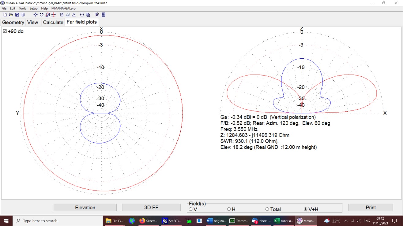
Figures 3a and 3b. MMANA-GAL calculations for the VGP

The 7 MHz VGP would have low resistance and high capacitive reactance on 3.5 MHz, typical of shortened antennas, with 777:1 VSWR. Radiation is vertically polarized with very low angle lobes (Figure 3a). On 10 MHz the VGP would have moderately high impedance, with 42:1 VSWR. The radiation is almost all vertically polarized, with some gain at higher angles (Figure 3b).

The VGP appeared to have better radiation patterns than the delta loop, so I tried using it on 3.5 and 10 MHz. I could get low VSWR by careful adjustment of the manual ATU, but did not get strong signal reports.

To design the matching networks, I needed to know the complex impedance of the antenna on those bands. This is a critical step, where a good measuring instrument is needed. I had problems using my nanoVNA at the antenna, but eventually measured impedances shown in Figure 4. Considering that the model was only an approximation of the actual antenna, the measured and modeled impedances were reasonably close. Using the measured values, I used the calculator TLDetails to estimate feedline losses.

The calculated losses of 9.1 dB and 5.8 dB in Figure 4 would explain the poor signal reports, but I began to wonder exactly what those numbers represented. Most hams know that transmission line loss increases with length, VSWR, and frequency, but on HF I never worried about losses because all my antennas have low VSWRs. I also use VHF/UHF and knew that there are high conductivity and dielectric losses at those frequencies, but now TLDetails calculated very high losses even at low frequencies, with a fairly short feedline. Over 90% of the total loss was called reflected loss, with small conductive and dielectric losses comprising the rest.

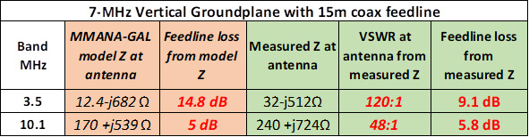
Figure 4. VGP impedance, VSWR, and feedline loss

Reflected power is still a hot topic

I was sleeping badly, wondering if so much power is really lost because of a mismatch. If it isn’t real, my time would be wasted building a remote matching unit.

As I read about reflected power and feedline loss, I found a memorable statement:

“Measurements made in the RF domain are steeped in tradition. Like most traditions, RF concepts are passed on by word of mouth as well as by written legend. Also like most traditions, the concepts are imperfectly understood by many who need to know better. In particular, the concept of forward and reflected power is often misunderstood.” – A Chief Technology Officer

It was comforting to know that I was not the only one confused. There seemed to be two main schools of thought, both surrounded by a swarm of misconceptions and confusion. A simple formula is used by TLDetails and other sources to calculate the reflected loss or mismatch loss (ML) from VSWR, based on reflected power canceling out some forward power. This ML equation is widely accepted, perhaps because it is so simple, but the logic seemed weak and I could not find good explanations of what happens to the lost power, or why cancellation occurs regardless of the phase difference between forward and reflected waves.

The opposite view was propounded in the 1970’s by Walter Maxwell, W2DU, a leading antenna expert. He wrote in QST magazine that VSWR was not as important as believed because the mismatch loss is completely made up when the line is matched at the transmitter, and all reflected power eventually goes out to the antenna and is radiated. The Maxwell side has been losing credibility, but occasionally scores a point by taking a shot at the ML equation.

An online argument started in 2017 with IZ2UUF’s blog, “The Myth of Reflected Power”, and continues to date. He showed by extensive lab bench tests that the ML equation is not generally applicable. TLDetails developer Dan McGuire, AC6LA, tried to clarify this, but did not change the formula. You might understand more if you read this blog and the many comments, or perhaps like me, you will understand less.

Common advice says it is fine to match at the rig when VSWR is under 3:1 because loss is low, but the gurus are silent if VSWR is much higher, such as the 10:1 or more I now expected. Some hams believe that reflected power is absorbed by the transmitter finals, so an ATU is needed at the rig to prevent damage, or that changing the length of coax will change the VSWR, or that the coax is “stressed” by high VSWR, while still others look down at hams who do not use expensive coaxial cable on HF. This is just a fraction of the misinformation circulating in the amateur community.

The more I read, the more confused I became. All the mathematics, elaborate graphics, pseudo-science, and laboratory demonstrations reminded me of the story of the three blind men who encountered an elephant, each describing it in his own incorrect way. I tossed and turned at night, still unsure if the feedline loss is real or not, but continued with the project so I could find out for myself.

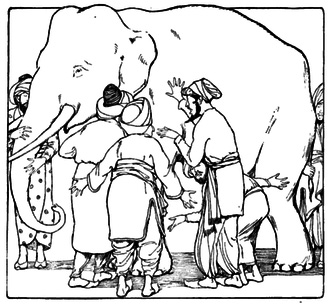
Figure 5. Confusion still reigns

Taming the L-network

Manual ATUs in the past used “T” and “pi” impedance matching networks with three or more reactive components. Simpler, less expensive L-networks are more limited in matching capability but are now used in many manual and most automatic ATUs.

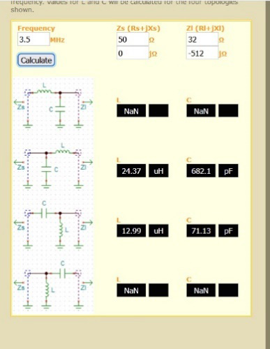
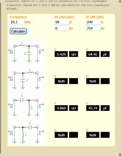
An L-network for a single frequency can be designed easily using one of the many online calculators. When the source and load impedances and the frequency are entered, inductance and capacitance values appear for the possible network topologies (Figures 6a and 6b).

Some more history

I love to build analog electronic gadgets. Along with the old transceiver and matching ATU, I brought back several boxes of old-school components to Okinawa and have used them to build several shack accessories. It brings me back to my teenage years when those parts were readily available and inexpensive. Many are now hard to find, such as variable capacitors, air coils and even half-watt carbon resistors. Some components and chassis pieces that JA9BB was apparently buying in installments were for a multiband transmitter. If any old-timers have information on this kit system, please contact me through FB NEWS.

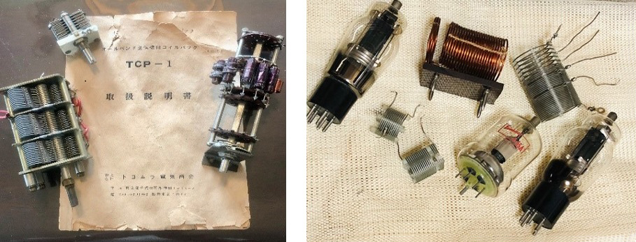
Figures 7a and 7b. Antique parts from JA9BB’s shack

Lessons learned (and not learned)

The shunt-C/series-L topology in Figures 6a and 6b called for very high L and C values on 3.5 MHz, but the other configuration used smaller components which I had on hand. For 10 MHz there was little difference between topologies.

From this point onward I ran into problems at almost every turn. Sometimes I felt like giving up, but I eventually found solutions to most of them.

• To start, I breadboarded a 10 MHz L-network and adjusted it for low VSWR with an analyzer at the antenna, but when I checked it at the rig, the match was slightly different. This also happens with my other antennas because of many coax jumpers and switches in the shack. A helper in the shack sent me video of the analyzer so I could adjust the networks on the roof in real time. I had to use this human remote tuning method several more times.
• Adjusting only the variable capacitor usually could not achieve an exact match because (as I learned) the Q factor is a third variable (with L and C) in some network equations. Since Q depends on the ratio of XL to XC, the inductance also needs to be adjustable. Automatic ATUs and roller coils in manual ATUs solve this problem of fine tuning, but it was difficult with my coils until I used the old technique of a ferrite “slug” on a threaded rod (Figure 11).
• I tried a shortcut that I hoped would shorten my clumsy experimentation. If an automatic tuner at the antenna found the correct tuning parameters, I could then substitute fixed components. My AT-100 did not have enough inductance to match very high impedance on 3.5 MHz, so I borrowed an MFJ-993 with a wider range and made a breadboard circuit to substitute L and C values (Figure 8). For reasons I still do not understand, I could not reproduce the automatic tuner’s results, so it was “back to Plan A.”

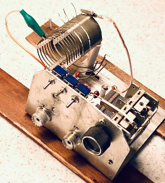
Figure 8. L/C substitution network (failed)

• I built the L-networks into a watertight box, with small relay modules to change the L and C for each band controlled from the shack (Figure 9a). I found it difficult to tune reliably because stray capacitances and inductances were nearly as high as the actual network parameters. I rewired it to switch each L-network as a unit (Figure 9b), and used open-frame DPDT relays with lower capacitance than the modules, reducing the number of relays.

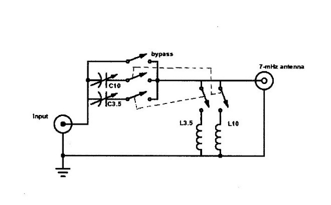
Figures 9a. Original and final network switching schemes

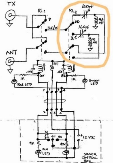
Figures 9b. Original and final network switching schemes

• I clearly hadn’t given enough attention to the layout and wiring, and soon I learned another lesson! The coax to the antenna exited from the top of the unit, and after a rainstorm I found that SO-239 (M) connectors are not watertight. With high humidity inside the box, the ordinary hookup wire I used failed spectacularly in several places when I tried high power (Figure 10). I calculated that peak RF voltage was as high as 1200 volts. I rewired it with better insulation and more direct routing, and moved the output coax to the bottom of the box (Figure 11). The 3.5 MHz variable capacitor had arced, so I repaired it and added a mica capacitor in series with it to reduce the voltage.

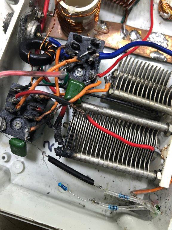
Figure 10. Rain released the magic smoke

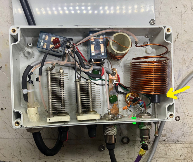
Figure 11. Final build with high-voltage wiring and ferrite slug tuning (arrow)

• The L-networks had to be adjusted with the unit connected to the antenna, which was difficult while balancing on a ladder in the hot sun. I built equivalent circuits of the VGP so I could make the adjustments on my workbench. The equivalent impedances gave VSWR sweeps through the matching unit that were identical to the actual antenna, and when I reconnected the adjusted unit to the antenna it was nearly perfectly tuned.

Figure 12. The 10 MHz (L) and 3.5 MHz (R) antenna equivalent circuits

And at last…

I had low VSWRs (<1.2:1) in the shack across the 10 MHz band and on the CW portion of 3.5 MHz (Figures 13a and b). The VGP was instantly tuned to either band or to 7 MHz by a switch on the operating desk. I could also switch quickly from the remote unit to the desktop ATU, maintaining the same VSWRs and forward power. This enabled easy “A/B” comparisons because the only difference was then the feedline loss (Figure 14).

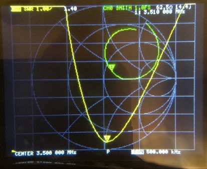
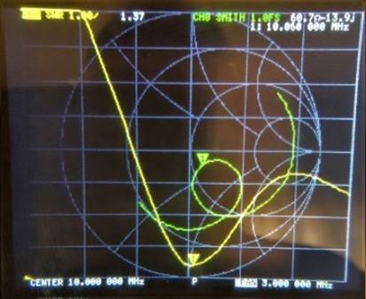
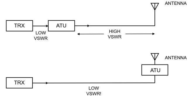
Figure 14. Desktop versus remote matching

Over several weeks of testing, comparison signal reports on 3.5 MHz from mainland Japan and nearby countries averaged two to four S-units better with the remote unit, and 7 to 10 dB better from Reverse Beacon Network spotters. On 10 MHz the average improvement in RBN spots was 2 to 3 dB. These on-air differences are very close to the calculated losses that were eliminated by the remote matching unit.

Figure 15. Waterproofed matching unit at the VGP feedpoint

Following this general approach to design and construction, a simple remote matching unit could be built inexpensively for as many bands as desired. As I look back on the months I spent on this project, it was much more difficult than I had expected, but I was richly rewarded by learning from my mistakes. Another bonus is that I can confidently discuss real-world results if I am ever drawn into the never-ending debate over reflected power loss.